Bayesian Fermi Estimation with `fermi`: The Chicago Piano Tuners Example • fermi

Introduction

The fermi package supports Bayesian Fermi estimation: breaking down uncertain quantities into components (decomposition), expressing beliefs as probability distributions (priors), and building uncertainty into the final estimates.

This vignette demonstrates the classic Fermi problem: > How many piano tuners are in Chicago?

We will:

Decompose the problem.
Construct expert-driven priors.
Run a Bayesian Fermi simulation.
Summarise and visualise the resulting distribution.

library(fermi)

How many piano tuners are in Chicago?

If you didn’t have access to data, how would you estimate the number of piano tuners in Chicago? A Fermi estimate breaks the problem into smaller components that can be estimated more easily. We then combine these estimates to get a final answer.

A Bayesian version of this approach encodes uncertainty about each component as a probability distribution (a prior). We then use Monte Carlo simulation to propagate this uncertainty through the calculation, resulting in a probability distribution for the final estimate.

First, we need to decompose the problem by breaking it down into smaller parts.

The decomposition we will use is:

$\text{tuners} = \frac{ \text{population} }{ \text{people per household} } \times \text{fraction of households with a piano} \times \text{tunings per piano per year} \;\Big/\; \left( \text{working days per year} \times \text{tunings per tuner per day} \right).$

Prior beliefs from expert judgement

Population of Chicago

Belief: 80% probability between 2.5M and 3.5M.

We’ll encode this belief as a gamma prior using the expert_gamma_prior() function. We are using a gamma distribution here because the population is a positive count.

population_prior <- expert_gamma_prior(
  q = c(2.5e6, 3.5e6),
  p = c(0.1, 0.9)
)
#> Warning in expert_gamma_prior(q = c(2500000, 3500000), p = c(0.1, 0.9)):
#> expert_gamma_prior: quantile match may be imprecise. Squared error on q:
#> 2.39e+08 (method = normal, shape ~= 59.1)
population_prior
#> fermi prior
#>   Distribution: gamma 
#>   Source      : expert 
#>   Parameters  :
#> $shape
#> [1] 59.12548
#> 
#> $rate
#> [1] 1.970849e-05

Let’s check expert_gamma_prior() has captured our beliefs correctly:

stats::qgamma(
  c(0.1, 0.9),
  shape = population_prior$params$shape,
  rate = population_prior$params$rate
)
#> [1] 2512119 3509602

Household size

Belief: Mean ≈ 2.7; 80% probability between 2.2 and 3.2.

We’ll encode this belief as a normal prior using the expert_normal_prior() function. We are using a normal distribution here because household size can be reasonably approximated as a continuous variable.

hh_size_prior <- expert_normal_prior(
  mean = 2.7,
  lower = 2.2,
  upper = 3.2,
  level = 0.8
)

hh_size_prior
#> fermi prior
#>   Distribution: normal 
#>   Source      : expert 
#>   Parameters  :
#> $mean
#> [1] 2.7
#> 
#> $sd
#> [1] 0.3901521

Fraction of households with a piano

Belief: 80% probability between 2% and 8%.

We’ll encode this belief as a beta prior using the expert_beta_prior() function. We are using a beta distribution here because the fraction is a probability between 0 and 1.

piano_frac_prior <- expert_beta_prior(
  q = c(0.02, 0.08),
  p = c(0.1, 0.9)
)

piano_frac_prior
#> fermi prior
#>   Distribution: beta 
#>   Source      : expert 
#>   Parameters  :
#> $shape1
#> [1] 3.623535
#> 
#> $shape2
#> [1] 72.7708

Let’s check expert_beta_prior() has captured our beliefs correctly:

stats::qbeta(
  c(0.1, 0.9),
  shape1 = piano_frac_prior$params$shape1,
  shape2 = piano_frac_prior$params$shape2
)
#> [1] 0.02000001 0.07999992

Tunings per piano per year

Belief: Most pianos tuned every 1–3 years ⇒ 0.3–1.0 tunings/year.

We’ll encode this belief as a gamma prior using the expert_gamma_prior() function. Again, we use a gamma distribution because the number of tunings is a positive count.

tunes_per_piano_prior <- expert_gamma_prior(
  q = c(0.3, 1.0),
  p = c(0.1, 0.9)
)

tunes_per_piano_prior
#> fermi prior
#>   Distribution: gamma 
#>   Source      : expert 
#>   Parameters  :
#> $shape
#> [1] 4.890221
#> 
#> $rate
#> [1] 7.851207

Working days per year

Belief: Mean ≈ 230; 90% probability between 180 and 280.

We’ll encode this belief as a normal prior using the expert_normal_prior() function. We are using a normal distribution here because the number of working days can be reasonably approximated as a continuous variable.

work_days_prior <- expert_normal_prior(
  mean = 230,
  lower = 180,
  upper = 280,
  level = 0.9
)

work_days_prior
#> fermi prior
#>   Distribution: normal 
#>   Source      : expert 
#>   Parameters  :
#> $mean
#> [1] 230
#> 
#> $sd
#> [1] 30.39784

Tunings per tuner per day

Belief: 80% probability of between 2 and 5 tunings per tuner per day.

We’ll encode this belief as a gamma prior using the expert_gamma_prior() function. Again, we use a gamma distribution because the number of tunings is a positive count.

tunes_day_prior <- expert_gamma_prior(
  q = c(2, 5),
  p = c(0.1, 0.9)
)

tunes_day_prior
#> fermi prior
#>   Distribution: gamma 
#>   Source      : expert 
#>   Parameters  :
#> $shape
#> [1] 8.187309
#> 
#> $rate
#> [1] 2.40024

Simulate the number of piano tuners (with uncertainty)

With our priors in place, we can now simulate over all components. The function passed to bf_fermi_simulate() mirrors the decomposition above.

tuner_draws <- bf_fermi_simulate(
  components = list(
    pop = population_prior,
    hh_size = hh_size_prior,
    piano_frac = piano_frac_prior,
    tunes_per_piano = tunes_per_piano_prior,
    work_days = work_days_prior,
    tunes_day = tunes_day_prior
  ),
  fun = function(
    population,
    hh_size,
    piano_frac,
    tunes_per_piano,
    work_days,
    tunes_day
  ) {
    (population / hh_size) *
      piano_frac *
      tunes_per_piano /
      (work_days * tunes_day)
  },
  n_draws = 20000
)

Summarise the result

We’ll summarise the results of the simulation (the posterior distribution) using posterior_summary().

tuner_summary <- posterior_summary(tuner_draws, cred_level = 0.89)
tuner_summary
#> Posterior summary
#>   Credible level: 89 %
#>   Median        : 36.31656 
#>   CI            : [8.606157, 129.9963]
#>   HDI           : [1.717152, 96.42675]

Based on our beliefs, and our uncertainty about them, we estimate there are around 36 piano tuners in Chicago, with a 89% credible interval from about 9 to 130.

Visualise the result

Finally, take a quick look at the posterior distribution. The dashed line marks the median; dotted lines are the 90% credible interval.

plot_posterior(tuner_draws, cred_level = 0.9)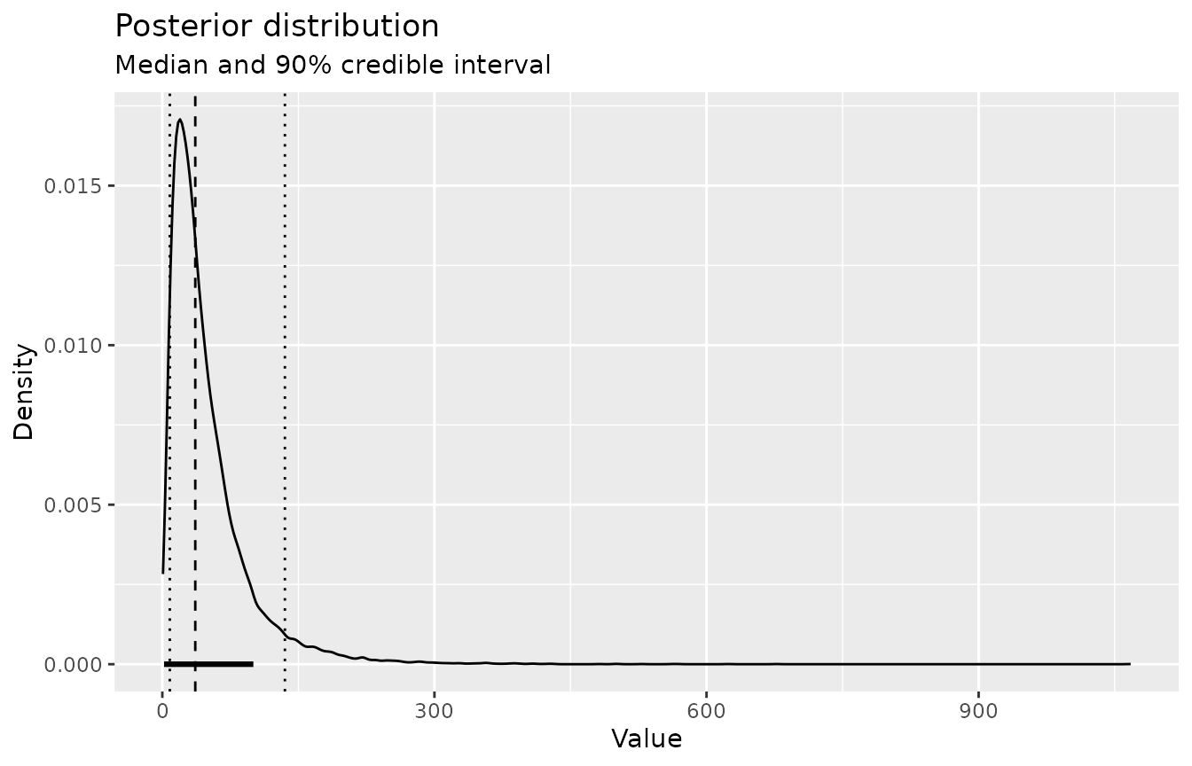

Conclusion

This vignette showed how to:

Decompose a Fermi problem,
Construct expert-driven Bayesian priors,
Simulate the resulting distribution using bf_fermi_simulate(),
Summarise and plot the implied number of piano tuners.

The same workflow applies to any Bayesian Fermi estimation task: break the problem into factors, elicit priors, and let simulation propagate the uncertainty.

This package also lets you fit priors to actual data, using fit_beta_prior(), fit_gamma_prior() and fit_normal_prior(). You can also update priors (e.g. based on expert beliefs) with data using conjugate Bayesian updating functions like beta_binom_posterior() and gamma_poisson_posterior(). See the package documentation for more details.